GANs

Notes about GANs from vanilla GAN to CycleGAN and StyleGAN.

(Vanilla) GAN

In short:

• Generator $G$ - tries to generate realistic looking images (maximize $D(G(z))$).
• Discriminator $D$ - tries to distinguish between real and generated images (minimize $D(G(z))$ and maximize $D(x)$). Discriminator makes for learned loss function for generator.
• The original GAN uses binary cross-entropy loss.
• Discriminator has softmax at the end and outputs values between $[0, 1]$ (0 - fake, 1 - real).
• Best for Generator is for the Discriminator to output ~0.5, which means that D can't tell if an image is real or fake (Nash equilibrium).
• Loss isn't interpretable because both the generator and discriminator can improve in the same time, so even if G's image quality improves, the loss can stay the same.

note

The original GAN from 2014 used MLP layers instead of Conv layers.

DCGAN

The simplest GAN that doesn't use FFN layers but Conv layers, takes a noise vector and gradually increases it through TransposeConv2d.

• Use conv layers instead of FFN layers.
• Use conv with a larger stride instead of pooling.
• Use batchnorm.
• ReLU in $G$ and LeakyReLU in $D$.
• $\beta_1=0.5$ (PyTorch default is $0.9$)

cGAN - Conditional GAN

Refers to the general idea of adding class information to the GAN. In the context of the Generator, this usually involves adding labels to the noise (concatenating two vectors). The Discriminator checks if the image is real or fake, having additional information about the class. (The Discriminator returns a scalar for each image).

# Adding conditioning in the Generator
def forward(x, y):
	cond = self.embedding(y)
	x = torch.cat([x, cond], dim=1) # x.shape = [bs, z_dim], cond.shape = [bs, embed_dim]
	return self.backbone(x)

# Adding conditioning in the Discriminator
def forward(x, y):
	out = self.net(x)
  cond = self.embed(y)
  return (x*y).sum(dim=[1, 2, 3])

note

There is also Projection Discriminator as a better conditioning method.

acGAN (Auxiliary Classifier GAN)

In acGAN, the discriminator has two outputs: one for real/fake (as in cGAN) and one for classifying the class. The Discriminator doesn't receive classes as input because it has to predict them.

# Discriminator (Generator remains the same as in cGAN)
def forward(self, img):
  features = self.model(img)
  validity = self.real_fake_head(features)
  class_logits = self.class_head(features)
  return validity, class_logits
  
loss_fn_bce = nn.BCELoss()  # For real/fake
loss_fn_ce = nn.CrossEntropyLoss()  # For classification

for i in range(epochs):
	# ...
	# Discriminator
	d_loss_real = loss_fn_bce(real_validity, torch.ones_like(real_validity)) + \\
	              loss_fn_ce(real_class_logits, real_labels)
	d_loss_fake = loss_fn_bce(fake_validity, torch.zeros_like(fake_validity)) + \\
	              loss_fn_ce(fake_class_logits, labels)
	d_loss = d_loss_real + d_loss_fake
	# ...
	# Generator
	g_loss_validity = loss_fn_bce(fake_validity, torch.ones_like(fake_validity))
	g_loss_class = loss_fn_ce(fake_class_logits, labels)
	g_loss = g_loss_validity + g_loss_class
  # ...

WGAN & WGAN-GP (Wasserstein GAN with Gradient Penalty)

Change of JS divergence (from Vanilla GAN) to Earth Mover Distance (aka Wasserstein distance).

• JS divergence works badly if two distributions have small or no overlap (mode collapse, vanishing grads).
• Wasserstein distance measures the "cost" of transforming one distribution into another, works even if there is no overlap between distributions, and gives meaningful values (decreasing loss of the discriminator says that Generator improves in quality).

In the original WGAN (without GP), weights are clipped (not the gradient) to ensure Lipschitz continuity. The parameter $c$ decides how strong the clipping is.

The purpose of the gradient penalty is to keep the critic in the space of 1-Lipschitz functions, so that the critic provides high-quality gradients and the Wasserstein distance is estimated better. (GP only for the critic).

LSGAN (Least Squares GAN)

Using L2 loss instead of BCE loss to calculate the loss:

$$\begin{align*} & loss_{fake} = (D(G(z)) - 0)^2 \\ & loss_{real} = (D(x) - 1)^2 \end{align*}$$

Progressive Growing GAN

The Generator is gradually trained, first at a low resolution, and a new layer that increases the resolution is added periodically. Advantages:

• Training stability: Starting with small images causes the model to learn the most important features of the image (shapes, colors) at the beginning, rather than textures and background details. This reduces the risk of training derailment.
• Training speed: Training on small images is much cheaper, and the model quickly adapts to a higher resolution.
• Better image quality.

Pix2Pix

An architecture created for img2img translation (e.g., sketch → image). The most important features are the use of adversarial loss + L1 loss (they didn't use L2 because of lower outlier resistance) and the introduction of PatchGAN (image discrimination with tiles instead of a scalar for the entire image - more detailed/local feedback for G).

Loss

• L1 for adhering to the outline but blurred (low-freq structure).
• Adv. loss is responsible for sharp edges (high-freq structure).

Model structure and other details

• UNet for the generator.
• PatchGAN - discrimination with tiles.
• Block structure: Conv + BatchNorm + ReLU.
• Dropout as a form of result diversity (enabled during inference; no noise vector as a source of randomness and diverse outputs).
• LR for D is 2x smaller than for G.
• Adam with b1=0.5 and b2=0.999.

CycleGAN

The CycleGAN architecture was made for style-transfer without needing special data for mapping $(A \rightarrow B)$. To achieve this, it uses a combination of 3 losses:

1. Cycle-consistency loss

Transforms an image into something and back, and compares the difference between the original and the generated one (the circle/cycle closes).

$$\begin{align*} &A \to G_1(A) \to B' \to G_2(B') \to A' \\ &\text{CycleLoss}_1 = ||A - A'|| \\ \\ &B \to G_2(B) \to A' \to G_1(A') \to B' \\ &\text{CycleLoss}_2 = ||B - B'|| \\ \\ &\text{CycleLoss}_{total} = \text{CycleLoss}_1 + \text{CycleLoss}_2 \end{align*}$$

2. Adversarial loss

The usual loss from the discriminator (each G has its own D).

3. Identity loss

The Generator sometimes receives an image that it should generate, so it shouldn't change anything in it, just return it (a form of regularization).

Features

• 2 generators and 2 discriminators.
• Doesn't need a dataset consisting of image pairs (it can be 2 arbitrary datasets from different domains, e.g., photos and paintings).
• Generators as autoencoders, not UNets (unlike Pix2Pix).
• Uses PatchGAN from Pix2Pix in the generator.

R3GAN

Summary

Authors developed a new loss function that has mathematical guarantees of convergence and is stable. With stable training achieved, they modify the architecture (starting from StyleGAN2), remove all the now-superfluous tricks, and modernize the architecture. Ultimately, they arrive at a stable and simpler GAN architecture that rivals previous GANs and diffusion-based SOTA models.

Details

1. Re-formulated Loss: Instead of calculating losses for D and G separately, they are combined.

   • Traditional GAN Loss:

     $L(\theta, \psi) = \mathbb{E}_{z \sim p_z} \left[ f \left( D_\psi(G_\theta(z)) \right) \right] + \mathbb{E}_{x \sim p_D} \left[ f \left( -D_\psi(x) \right) \right]$ G and D are calculated separately, causing real and fake samples to be far apart (D pushes them apart).

   • "Relativistic" GAN Loss:

     $L(\theta, \psi) = \mathbb{E}_{z \sim p_z, \ x \sim p_D} \left[ f \left( D_\psi(G_\theta(z)) - D_\psi(x) \right) \right]$ Here, G and D are linked. D evaluates the "realness" relative to real samples, so fake samples should always be in the vicinity of real samples.

2. Addition of Zero-Centered Gradient Penalties (R1 and R2):

   • R1: Penalizes the gradient magnitudes of D on real samples.
   • R2: Penalizes the gradient magnitudes of D on fake samples.

   The goal is to reduce the gradients for G when it's close to generating real samples (eliminating training oscillations). When $p_{fake} = p_{real}$, the gradients from D should be 0.

3. Simplification and Modernization of the Architecture: They start with StyleGAN2 and remove everything that was added to increase stability and convergence. Then, they change the architecture to ResNeXt, but without normalization, because they use Fixup initialization, which doesn't require it.

StyleGAN

A complex architecture that has many tricks to achieve stable training and good quality. Allows for interpolation between any two images. Many versions of StyleGAN have been released. In a nutshell:

1. The $z$ noise vector is transformed by the Mapping network into the vector $w$ (latent code).
2. The Synthesis network starts creating an image from a learnable tensor 4x4 (Const 4x4x512).
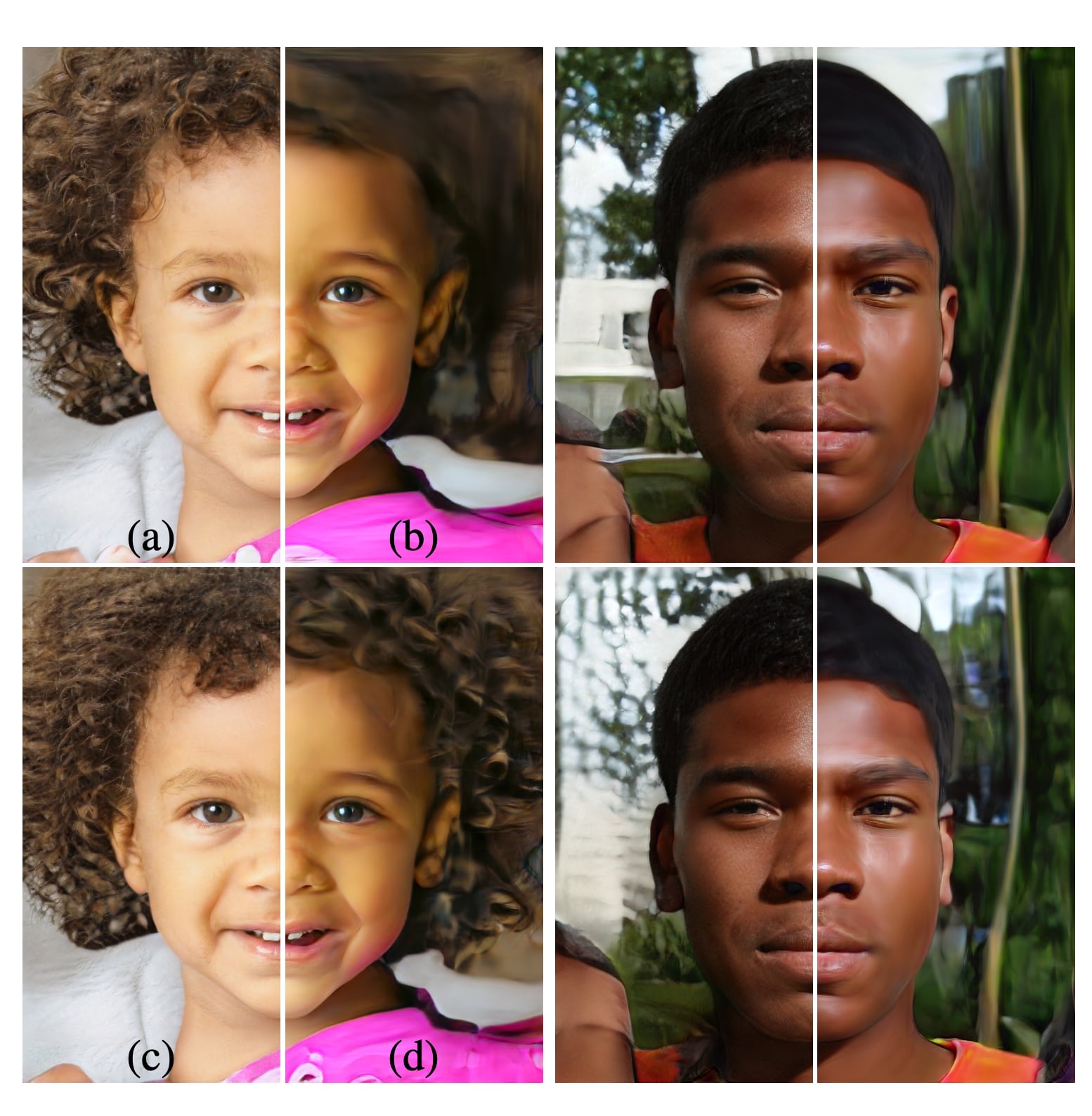
3. The gradually upsampled feature map passes through subsequent blocks into which the latent code $w$ (through AdaIN - a type of normalization) and the noise vector $B$ are injected.

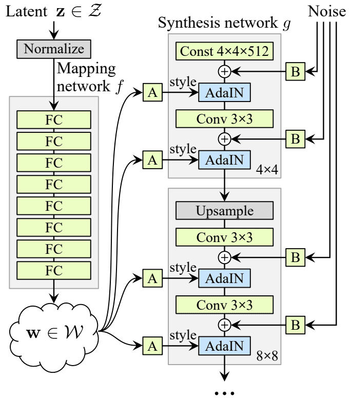
Injecting noise through $B$ adds high-frequency details to the image (left with noise, right without noise).

Other stuff (tips, tricks, minor papers)

Gated Shortcut (arXiv:2201.11351)

The Gated shortcut decides what remains from the residual stream and what is added from the features. Used only in the Generator. $f_i$ - input $f_c$ - feature (what's on the output of conv, bn, relu) $f_o$ - output $*$ - conv, $\odot$ - concat, $\otimes$ - element-wise multiplication

1. $f_g = \text{sigmoid}(\text{conv}(f_c \odot f_i))$ - gate, value 0-1
2. $f_r = \text{conv}(f_c \odot f_i)$ - refinement, learned transformation of combined features; what to add
3. $f_o = \text{conv}[f_g \otimes f_c + (1-f_g) \otimes f_r]$ here: $f_g \otimes f_c$ means how much to take from the feature based on $f_i$ and $f_c$. $(1-f_g) \otimes f_r$ means the rest, which comes from the combination of $f_i$ and $f_c$.

Authors claims that it's better than other gated residuals because it can better add/remove data from the residual stream/features ($f_{EGS}$ is other way to implement a gated shortcut): $f_{EGS} = f_g \otimes f_i + (1-f_g) \otimes f_c$

In Eq. 6, $f_{EGS}$ can be interpreted as the weighted summation of the $f_i$ and $f_c$, where weight value is $f_g$. Thus, if $f_g$ is 0.5, it is equal to the scaled-identity shortcut; it cannot effectively keep (or remove) the relevant (or irrelevant) information in $f_c$. In contrast, instead of directly summing $f_i$, the proposed method produces the refinement feature, i.e. $f_r$.

This can probably be used in other architectures. The gating mechanism doesn't have to be useful only for GANs (e.g., LSTM).

Checkerboard Artifacts

Transposed conv with overlapping stride can cause checkerboard artifacts - solution: use regular Conv2d + Upsampling2d("nearest"); then conv can overlap.